Show the code
pacman::p_load(sf, sfdep, tmap, tidyverse, knitr, plotly)TASK :- Weekday morning peak (Period: 6am to 9am)
Chia Yong Soon
November 26, 2023
December 2, 2023
Setting the Scene As city-wide urban infrastructures such as buses, taxis, mass rapid transit, public utilities and roads become digital, the datasets obtained can be used as a framework for tracking movement patterns through space and time. This is particularly true with the recent trend of massive deployment of pervasive computing technologies such as GPS and RFID on the vehicles. For example, routes and ridership data were collected with the use of smart cards and Global Positioning System (GPS) devices available on the public buses. These massive movement data collected are likely to contain structure and patterns that provide useful information about characteristics of the measured phenomena. The identification, analysis and comparison of such patterns will provide greater insights on human movement and behaviours within a city. These understandings will potentially contribute to a better urban management and useful information for urban transport services providers both from the private and public sector to formulate informed decision to gain competitive advantage.
In real-world practices, the use of these massive locational aware data, however, tend to be confined to simple tracking and mapping with GIS applications. This is mainly due to a general lack of functions in conventional GIS which is capable of analysing and model spatial and spatio-temporal data effectively.
Objectives Exploratory Spatial Data Analysis (ESDA) hold tremendous potential to address complex problems facing society. In this study, you are tasked to apply appropriate Local Indicators of Spatial Association (GLISA) and Emerging Hot Spot Analysis (EHSA) to undercover the spatial and spatio-temporal mobility patterns of public bus passengers in Singapore.
With reference to the time intervals provided in the table below, compute the passenger trips generated by origin at the hexagon level.
| Peak hour period | Bus tap on time |
|---|---|
| Weekday morning peak | 6am to 9am |
| Weekday afternoon peak | 5pm to 8pm |
| Weekend/holiday morning peak | 11am to 2pm |
| Weekend/holiday evening peak | 4pm to 7pm |
Display the geographical distribution of the passenger trips by using appropriate geovisualisation methods,
Describe the spatial patterns revealed by the geovisualisation (not more than 200 words per visual).
Six R packages will be used for this exercise, they are sf, sfdep, tmap, tidyverse, knitr, plotly.
sf: Purpose: The sf package stands for “simple features” and is used for working with spatial data in R. It provides a framework for representing and manipulating geometric objects like points, lines, and polygons, making it useful for tasks such as geographic information system (GIS) analysis.
sfdep: Purpose: The sfdep provides users with a way to conduct “Exploratory Spatial Data Analysis”, typical for exploratory data analysis. It evaluates the phenomena captured in the data on whether they are dependent upon space–or are spatially auto-correlated. “Local Indicators of Spatial Association”, LISAs for short are measures that are developed to identify whether some observed pattern is truly random or impacted by its relationship in space.
tmap: Purpose: tmap is a package for creating thematic maps in R. It provides a simple and consistent interface for visualizing spatial data, making it easier to create informative and visually appealing maps. It is often used in conjunction with the sf package for handling spatial data.
tidyverse: Purpose: The tidyverse is not a single package but a collection of R packages that work together cohesively for data manipulation and visualization. It includes popular packages like ggplot2 for plotting, dplyr for data manipulation, tidyr for data tidying, and others. The tidyverse philosophy emphasizes a consistent and intuitive approach to data analysis.
knitr: Purpose: knitr is a package for dynamic report generation in R. It allows you to embed R code directly into documents and then render the code and its output, such as tables and plots, into various document formats like HTML, PDF, or Word. It is commonly used with R Markdown to create reproducible research reports.
plotly: Purpose: plotly is a package for creating interactive and dynamic plots in R. It supports a variety of chart types, including scatter plots, line charts, and 3D plots. The resulting visualizations can be embedded into web pages, making it a powerful tool for creating interactive and shareable data visualizations.
For the purpose of this take-home exercise, Passenger Volume by Origin Destination Bus Stops downloaded from LTA DataMall will be used.
Since listings data set is in csv file format, we will use read_csv() of readr package to import origin_destination_bus.csv as shown the code chunk below. The output R object is called odbus1023 and it is a tibble data frame.
Rows: 5694297 Columns: 7
── Column specification ────────────────────────────────────────────────────────
Delimiter: ","
chr (5): YEAR_MONTH, DAY_TYPE, PT_TYPE, ORIGIN_PT_CODE, DESTINATION_PT_CODE
dbl (2): TIME_PER_HOUR, TOTAL_TRIPS

ℹ Use `spec()` to retrieve the full column specification for this data.
ℹ Specify the column types or set `show_col_types = FALSE` to quiet this message.
A quick check of odbus tibble data frame shows that the values in OROGIN_PT_CODE and DESTINATON_PT_CODE are in numeric data type.
Rows: 5,694,297
Columns: 7
$ YEAR_MONTH          <chr> "2023-10", "2023-10", "2023-10", "2023-10", "2023-…
$ DAY_TYPE            <chr> "WEEKENDS/HOLIDAY", "WEEKDAY", "WEEKENDS/HOLIDAY",…
$ TIME_PER_HOUR       <dbl> 16, 16, 14, 14, 17, 17, 17, 7, 14, 14, 10, 20, 20,…
$ PT_TYPE             <chr> "BUS", "BUS", "BUS", "BUS", "BUS", "BUS", "BUS", "…
$ ORIGIN_PT_CODE      <chr> "04168", "04168", "80119", "80119", "44069", "2028…
$ DESTINATION_PT_CODE <chr> "10051", "10051", "90079", "90079", "17229", "2014…
$ TOTAL_TRIPS         <dbl> 3, 5, 3, 5, 4, 1, 24, 2, 1, 7, 3, 2, 5, 1, 1, 1, 1…
Convert these data values into factor data type.
Notice that both of them are in factor data type now.
Rows: 5,694,297
Columns: 7
$ YEAR_MONTH          <chr> "2023-10", "2023-10", "2023-10", "2023-10", "2023-…
$ DAY_TYPE            <chr> "WEEKENDS/HOLIDAY", "WEEKDAY", "WEEKENDS/HOLIDAY",…
$ TIME_PER_HOUR       <dbl> 16, 16, 14, 14, 17, 17, 17, 7, 14, 14, 10, 20, 20,…
$ PT_TYPE             <chr> "BUS", "BUS", "BUS", "BUS", "BUS", "BUS", "BUS", "…
$ ORIGIN_PT_CODE      <fct> 04168, 04168, 80119, 80119, 44069, 20281, 20281, 1…
$ DESTINATION_PT_CODE <fct> 10051, 10051, 90079, 90079, 17229, 20141, 20141, 1…
$ TOTAL_TRIPS <dbl> 3, 5, 3, 5, 4, 1, 24, 2, 1, 7, 3, 2, 5, 1, 1, 1, 1…For the purpose of extracting the commuting flows during the weekday morning peak for the period from 6am to 9am. Call the output tibble data table as origin_WDMP_6_9.
| Peak hour period | Bus tap on time |
|---|---|
| Weekday morning peak | 6am to 9am |
View the top few rows of the summarized trips by ORIGIN_PT_CODE.
# A tibble: 6 × 2
  ORIGIN_PT_CODE TRIPS
  <fct>          <dbl>
1 01012           1770
2 01013            841
3 01019           1530
4 01029           2483
5 01039           2919
6 01059           1734
We will save the output in rds format for future used.
The code chunk below will be used to import the save origin_WDMP_6_9.rds into R environment.
Two geospatial data will be used in this study, they are:
Bus Stop Location from LTA DataMall. It provides information about all the bus stops currently being serviced by buses, including the bus stop code (identifier) and location coordinates.
hexagon, a hexagon layer of 250m (this distance is the perpendicular distance between the centre of the hexagon and its edges.) should be used to replace the relative coarse and irregular Master Plan 2019 Planning Sub-zone GIS data set of URA.
In this section, you are required to import two shapefile into RStudio, they are: - BusStop: This data provides the location of bus stop as at 2nd quarter of 2023. - MPSZ-2019: This data provides the sub-zone boundary of URA Master Plan 2019.
The code chunk below uses st_read() function of sf package to import BusStop shapefile into R as line feature data frame.
Reading layer `BusStop' from data source
  `C:\chiays\ISS624\Take-home_Ex\Take-home_Ex1\data\geospatial'
  using driver `ESRI Shapefile'
Simple feature collection with 5161 features and 3 fields
Geometry type: POINT
Dimension:     XY
Bounding box:  xmin: 3970.122 ymin: 26482.1 xmax: 48284.56 ymax: 52983.82
Projected CRS: SVY21
The message above reveals that there are a total of 5161 features and 3 fields in BusStop linestring feature data frame and it is in svy21 projected coordinates system too.
The structure of busstop sf tibble data frame should look as below.
Rows: 5,161
Columns: 4
$ BUS_STOP_N <chr> "22069", "32071", "44331", "96081", "11561", "66191", "2338…
$ BUS_ROOF_N <chr> "B06", "B23", "B01", "B05", "B05", "B03", "B02A", "B02", "B…
$ LOC_DESC   <chr> "OPP CEVA LOGISTICS", "AFT TRACK 13", "BLK 239", "GRACE IND…
$ geometry   <POINT [m]> POINT (13576.31 32883.65), POINT (13228.59 44206.38),…
Import MPSZ-2019 into RStudio and save it as a sf data frame called mpsz.
Reading layer `MPSZ-2019' from data source
  `C:\chiays\ISS624\Take-home_Ex\Take-home_Ex1\data\geospatial'
  using driver `ESRI Shapefile'
Simple feature collection with 332 features and 6 fields
Geometry type: MULTIPOLYGON
Dimension:     XY
Bounding box:  xmin: 103.6057 ymin: 1.158699 xmax: 104.0885 ymax: 1.470775
Geodetic CRS: WGS 84The structure of mpsz sf tibble data frame should look as below.
Rows: 332
Columns: 7
$ SUBZONE_N  <chr> "MARINA EAST", "INSTITUTION HILL", "ROBERTSON QUAY", "JURON…
$ SUBZONE_C  <chr> "MESZ01", "RVSZ05", "SRSZ01", "WISZ01", "MUSZ02", "MPSZ05",…
$ PLN_AREA_N <chr> "MARINA EAST", "RIVER VALLEY", "SINGAPORE RIVER", "WESTERN …
$ PLN_AREA_C <chr> "ME", "RV", "SR", "WI", "MU", "MP", "WI", "WI", "SI", "SI",…
$ REGION_N   <chr> "CENTRAL REGION", "CENTRAL REGION", "CENTRAL REGION", "WEST…
$ REGION_C   <chr> "CR", "CR", "CR", "WR", "CR", "CR", "WR", "WR", "CR", "CR",…
$ geometry <MULTIPOLYGON [m]> MULTIPOLYGON (((33222.98 29..., MULTIPOLYGON (…Code chunk below populates the planning subzone code (i.e. SUBZONE_C) of mpsz sf data frame into busstop sf data frame.
Warning: attribute variables are assumed to be spatially constant throughout
all geometries
Before moving to the next step, save the output into rds format.
Next, append the planning subzone code from busstop_mpsz data frame onto origin_WDMP_6_9 data frame.
Check for duplicate records
See if any duplicate records.
Rows: 26
Columns: 3
$ ORIGIN_BS <fct> 11009, 11009, 22501, 22501, 43709, 43709, 47201, 47201, 5107…
$ TRIPS     <dbl> 17311, 17311, 11384, 11384, 1329, 1329, 25910, 25910, 6698, …
$ ORIGIN_SZ <chr> "QTSZ01", "QTSZ01", "JWSZ09", "JWSZ09", "BKSZ07", "BKSZ07", …As shown above, there is none. Nonetheless, we can remove duplicate records (if any) with the following code.
Next, write a code chunk to update od_data data frame with the planning subzone codes.
Warning in sf_column %in% names(g): Detected an unexpected many-to-many relationship between `x` and `y`.
ℹ Row 149 of `x` matches multiple rows in `y`.
ℹ Row 3044 of `y` matches multiple rows in `x`.
ℹ If a many-to-many relationship is expected, set `relationship =
"many-to-many"` to silence this warning.Prepare a choropleth map showing the distribution of passenger trips at planning sub-zone level.
tm_shape(origintrip_SZ_HEX)+
  tm_symbols(size = 0.5)+
  tm_layout(main.title = "Passenger trips generated at planning sub-zone level",
            main.title.position = "center",
            main.title.size = 1.2,
            legend.height = 0.45,
            legend.width = 0.35,
            frame = TRUE) +

  tm_compass(type="8star", size = 2) +
  tm_scale_bar() +
  tm_grid(alpha =0.2) +
  tm_credits("Source: Planning Sub-zone boundary from URA\n and Passenger trips data from LTA",
             position = c("left", "bottom"))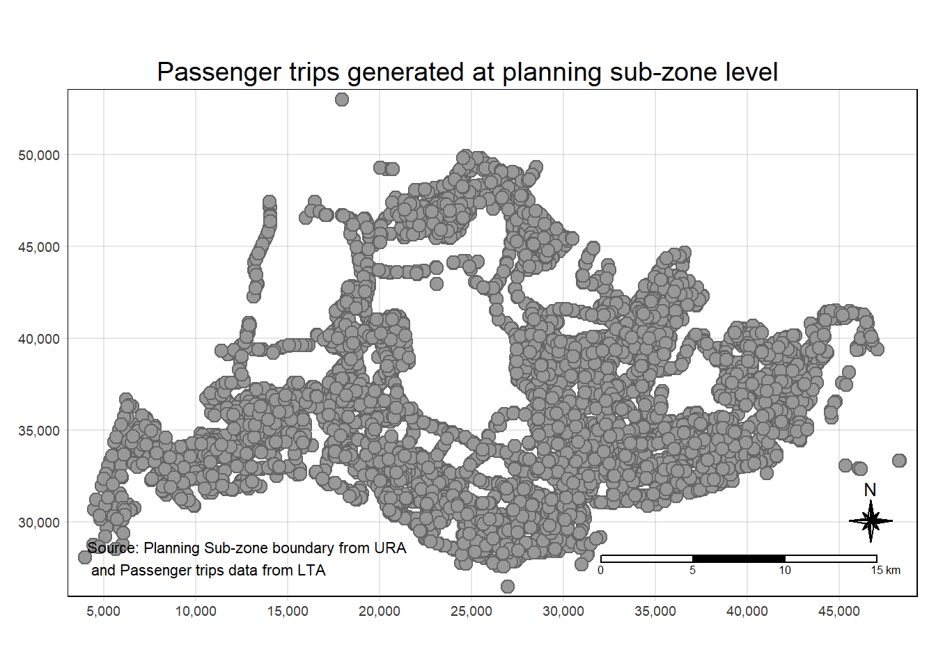
tm_shape(origintrip_SZ)+
  tm_fill("TOT_TRIPS",
          style = "quantile",
          palette = "Blues",
          title = "Passenger trips") +
  tm_layout(main.title = "Passenger trips generated at planning sub-zone level",
            main.title.position = "center",
            main.title.size = 1.2,
            legend.height = 0.45,
            legend.width = 0.35,
            frame = TRUE) +
  tm_borders(alpha = 0.5) +
  tm_compass(type="8star", size = 2) +
  tm_scale_bar() +
  tm_grid(alpha =0.2) +
  tm_credits("Source: Planning Sub-zone boundary from URA\n and Passenger trips data from LTA",
             position = c("left", "bottom"))
By and large, there are two types of spatial weights, they are contiguity weights and distance-based weights. In the steps below, I will apply contiguity spatial weights by using sfdep.
Two steps are required to derive a contiguity spatial weights, they are: a) identifying contiguity neighbour list by st_contiguity() of sfdep package, and b) deriving the contiguity spatial weights by using st_weights() of sfdep package
In the code chunk below st_contiguity() is used to derive a contiguity neighbour list by using Queen’s method.
The code chunk below is used to print the summary of the first lag neighbour list (i.e. nb) .
Neighbour list object:
Number of regions: 332
Number of nonzero links: 2002
Percentage nonzero weights: 1.816301
Average number of links: 6.03012
5 regions with no links:
7 8 9 304 317
6 disjoint connected subgraphs
Link number distribution:

 0  1  2  3  4  5  6  7  8  9 10 11 12 17
 5  2  5 10 28 75 90 54 38 17  3  2  1  2
2 least connected regions:
4 159 with 1 link
2 most connected regions:
273 300 with 17 links
The summary report above shows that there are 332 area units in Singapore. The most connected area units (i.e. 273 and 300) has 17 neighbours. The least connected area units (i.e. 4 and 159) has only one neighbour. There are also present of 5 areas with no links at all (i.e. 7, 8, 9, 304 and 317).
To view the content of the data table, you can either display the output data frame on RStudio data viewer or by printing out the first ten records by using the code chunk below.
Simple feature collection with 332 features and 8 fields
Geometry type: MULTIPOLYGON
Dimension:     XY
Bounding box:  xmin: 2667.538 ymin: 15748.72 xmax: 56396.44 ymax: 50256.33
Projected CRS: SVY21 / Singapore TM
First 10 features:
                         nb               SUBZONE_N SUBZONE_C       PLN_AREA_N
1         6, 36, 52, 70, 91             MARINA EAST    MESZ01      MARINA EAST
2              3, 5, 72, 75        INSTITUTION HILL    RVSZ05     RIVER VALLEY
3  2, 5, 37, 42, 43, 75, 86          ROBERTSON QUAY    SRSZ01  SINGAPORE RIVER
4                       119 JURONG ISLAND AND BUKOM    WISZ01  WESTERN ISLANDS
5  2, 3, 43, 71, 72, 73, 77            FORT CANNING    MUSZ02           MUSEUM
6        1, 52, 81, 94, 293        MARINA EAST (MP)    MPSZ05    MARINE PARADE
7                         0                  SUDONG    WISZ03  WESTERN ISLANDS
8                         0                 SEMAKAU    WISZ02  WESTERN ISLANDS
9                         0          SOUTHERN GROUP    SISZ02 SOUTHERN ISLANDS
10                   11, 14                 SENTOSA    SISZ01 SOUTHERN ISLANDS
   PLN_AREA_C       REGION_N REGION_C TOT_TRIPS                       geometry
1          ME CENTRAL REGION       CR         0 MULTIPOLYGON (((33222.98 29...
2          RV CENTRAL REGION       CR      7396 MULTIPOLYGON (((28481.45 30...
3          SR CENTRAL REGION       CR     24633 MULTIPOLYGON (((28087.34 30...
4          WI    WEST REGION       WR         0 MULTIPOLYGON (((14557.7 304...
5          MU CENTRAL REGION       CR      4909 MULTIPOLYGON (((29542.53 31...
6          MP CENTRAL REGION       CR         0 MULTIPOLYGON (((35279.55 30...
7          WI    WEST REGION       WR         0 MULTIPOLYGON (((15772.59 21...
8          WI    WEST REGION       WR         0 MULTIPOLYGON (((19843.41 21...
9          SI CENTRAL REGION       CR         0 MULTIPOLYGON (((30870.53 22...
10 SI CENTRAL REGION CR 40 MULTIPOLYGON (((26879.04 26...In the code chunk below st_contiguity() is used to derive a contiguity neighbour list by using Queen’s method.
Simple feature collection with 327 features and 7 fields
Geometry type: MULTIPOLYGON
Dimension:     XY
Bounding box:  xmin: 2667.538 ymin: 21448.47 xmax: 55941.94 ymax: 50256.33
Projected CRS: SVY21 / Singapore TM
First 10 features:
                 SUBZONE_N SUBZONE_C       PLN_AREA_N PLN_AREA_C       REGION_N
1              MARINA EAST    MESZ01      MARINA EAST         ME CENTRAL REGION
2         INSTITUTION HILL    RVSZ05     RIVER VALLEY         RV CENTRAL REGION
3           ROBERTSON QUAY    SRSZ01  SINGAPORE RIVER         SR CENTRAL REGION
4  JURONG ISLAND AND BUKOM    WISZ01  WESTERN ISLANDS         WI    WEST REGION
5             FORT CANNING    MUSZ02           MUSEUM         MU CENTRAL REGION
6         MARINA EAST (MP)    MPSZ05    MARINE PARADE         MP CENTRAL REGION
10                 SENTOSA    SISZ01 SOUTHERN ISLANDS         SI CENTRAL REGION
11          CITY TERMINALS    BMSZ17      BUKIT MERAH         BM CENTRAL REGION
12                   ANSON    DTSZ10    DOWNTOWN CORE         DT CENTRAL REGION
13            STRAITS VIEW    SVSZ01     STRAITS VIEW         SV CENTRAL REGION
   REGION_C TOT_TRIPS                       geometry
1        CR         0 MULTIPOLYGON (((33222.98 29...
2        CR      7396 MULTIPOLYGON (((28481.45 30...
3        CR     24633 MULTIPOLYGON (((28087.34 30...
4        WR         0 MULTIPOLYGON (((14557.7 304...
5        CR      4909 MULTIPOLYGON (((29542.53 31...
6        CR         0 MULTIPOLYGON (((35279.55 30...
10       CR        40 MULTIPOLYGON (((26879.04 26...
11       CR     13526 MULTIPOLYGON (((27891.15 28...
12       CR      9427 MULTIPOLYGON (((29201.07 28...
13 CR 686 MULTIPOLYGON (((31269.21 28...In the code chunk below, queen method is used to derive the contiguity weights.
Notice that st_weights() provides three arguments, they are:
Simple feature collection with 327 features and 9 fields
Geometry type: MULTIPOLYGON
Dimension:     XY
Bounding box:  xmin: 2667.538 ymin: 21448.47 xmax: 55941.94 ymax: 50256.33
Projected CRS: SVY21 / Singapore TM
First 10 features:
                             nb
1             6, 33, 49, 67, 88
2                  3, 5, 69, 72
3      2, 5, 34, 39, 40, 72, 83
4                           116
5      2, 3, 40, 68, 69, 70, 74
6            1, 49, 78, 91, 290
10                        8, 11
11 7, 9, 10, 11, 12, 14, 18, 21
12            8, 13, 14, 21, 25
13                8, 21, 30, 33
                                                                            wt
1                                                      0.2, 0.2, 0.2, 0.2, 0.2
2                                                       0.25, 0.25, 0.25, 0.25
3  0.1428571, 0.1428571, 0.1428571, 0.1428571, 0.1428571, 0.1428571, 0.1428571
4                                                                            1
5  0.1428571, 0.1428571, 0.1428571, 0.1428571, 0.1428571, 0.1428571, 0.1428571
6                                                      0.2, 0.2, 0.2, 0.2, 0.2
10                                                                    0.5, 0.5
11                      0.125, 0.125, 0.125, 0.125, 0.125, 0.125, 0.125, 0.125
12                                                     0.2, 0.2, 0.2, 0.2, 0.2
13                                                      0.25, 0.25, 0.25, 0.25
                 SUBZONE_N SUBZONE_C       PLN_AREA_N PLN_AREA_C       REGION_N
1              MARINA EAST    MESZ01      MARINA EAST         ME CENTRAL REGION
2         INSTITUTION HILL    RVSZ05     RIVER VALLEY         RV CENTRAL REGION
3           ROBERTSON QUAY    SRSZ01  SINGAPORE RIVER         SR CENTRAL REGION
4  JURONG ISLAND AND BUKOM    WISZ01  WESTERN ISLANDS         WI    WEST REGION
5             FORT CANNING    MUSZ02           MUSEUM         MU CENTRAL REGION
6         MARINA EAST (MP)    MPSZ05    MARINE PARADE         MP CENTRAL REGION
10                 SENTOSA    SISZ01 SOUTHERN ISLANDS         SI CENTRAL REGION
11          CITY TERMINALS    BMSZ17      BUKIT MERAH         BM CENTRAL REGION
12                   ANSON    DTSZ10    DOWNTOWN CORE         DT CENTRAL REGION
13            STRAITS VIEW    SVSZ01     STRAITS VIEW         SV CENTRAL REGION
   REGION_C TOT_TRIPS                       geometry
1        CR         0 MULTIPOLYGON (((33222.98 29...
2        CR      7396 MULTIPOLYGON (((28481.45 30...
3        CR     24633 MULTIPOLYGON (((28087.34 30...
4        WR         0 MULTIPOLYGON (((14557.7 304...
5        CR      4909 MULTIPOLYGON (((29542.53 31...
6        CR         0 MULTIPOLYGON (((35279.55 30...
10       CR        40 MULTIPOLYGON (((26879.04 26...
11       CR     13526 MULTIPOLYGON (((27891.15 28...
12       CR      9427 MULTIPOLYGON (((29201.07 28...
13       CR       686 MULTIPOLYGON (((31269.21 28...
Replace NA with 0
In the code chunk below, global_moran() function is used to compute the Moran’s I value. Different from spdep package, the output is a tibble data.frame.
List of 2
 $ I: num 0.254
 $ K: num 16.2
I: (Moran’s I): The Moran’s I value is a measure of spatial autocorrelation. It ranges from -1 to 1. A positive Moran’s I indicates positive spatial autocorrelation, meaning similar values are close to each other.
K: (Z-score): The z-score associated with Moran’s I is a measure of the significance of the spatial autocorrelation. A higher absolute z-score indicates a stronger departure from the null hypothesis (no spatial autocorrelation). Typically, if the absolute z-score is greater than 1.96 (for a 95% confidence level), the spatial autocorrelation is considered statistically significant.
Thus, result indicates positive spatial autocorrelation (clustering of similar values).
In general, Moran’s I test will be performed instead of just computing the Moran’s I statistics. With sfdep package, Moran’s I test can be performed by using global_moran_test() as shown in the code chunk below.
    Moran I test under randomisation

data:  x
weights: listw

Moran I statistic standard deviate = 8.1498, p-value < 2.2e-16
alternative hypothesis: greater
sample estimates:
Moran I statistic       Expectation          Variance
     0.2543190520     -0.0030674847      0.0009974257
p-value: < 2.2e-16 :- The p-value is associated with the Moran I statistic standard deviate. It indicates the probability of observing a Moran’s I statistic as extreme as the one calculated, assuming the null hypothesis (no spatial autocorrelation). A very small p-value (< 0.05) typically leads to rejecting the null hypothesis.
Alternative Hypothesis :- greater: The alternative hypothesis here is “greater,” suggesting that you are testing for positive spatial autocorrelation (clustering of similar values). Sample Estimates:
Based on the estimated values from the observed data:
Moran I Statistic: 0.2543 :- This is your observed Moran’s I statistic. It’s a measure of spatial autocorrelation. Values close to 1 indicate positive spatial autocorrelation (values clustered together).
Expectation: -0.0031 :- The expected value of Moran’s I under the null hypothesis of spatial randomness. It’s close to zero because, under the null hypothesis, there is no spatial autocorrelation. Variance: 0.0010
Given the very small p-value (p-value < 2.2e-16), it shows strong evidence to reject the null hypothesis, suggesting that there is significant positive spatial autocorrelation in the data.
In summary, the observed Moran’s I (0.2543) is significantly different from what would be expected under spatial randomness, indicating the presence of spatial autocorrelation. The positive sign suggests that similar values are clustered together in space.
In practice, monte carlo simulation should be used to perform the statistical test. For sfdep, it is supported by globel_moran_perm()
Use set.seed() before performing simulation to ensure that the computation is reproducible.
Next, global_moran_perm() is used to perform Monte Carlo simulation.
    Monte-Carlo simulation of Moran I

data:  x
weights: listw
number of simulations + 1: 100

statistic = 0.25432, observed rank = 100, p-value < 2.2e-16
alternative hypothesis: two.sided
Number of Simulations: 100 :- This indicates that a total of 100 Monte Carlo simulations were performed.
Statistic: 0.25432 :- This is the observed Moran’s I statistic from the original data.
Observed Rank: 100 :- The observed rank represents the rank of the observed statistic within the distribution of simulated statistics. In this case, the observed Moran’s I falls into the highest (or lowest, depending on the context) 100 out of the 100 + 1 simulated values.
p-value: < 2.2e-16 :- The p-value associated with the Monte Carlo simulation. It indicates the probability of observing a Moran’s I statistic as extreme as the one calculated, assuming the null hypothesis (no spatial autocorrelation). A very small p-value (< 0.05) typically leads to rejecting the null hypothesis.
Alternative Hypothesis: two.sided :- The alternative hypothesis here is “two-sided,” suggesting that the test for spatial autocorrelation is in general, without specifying a particular direction (positive or negative).
In summary, the very small p-value (< 2.2e-16) suggests strong evidence to reject the null hypothesis of no spatial autocorrelation. The output supports the conclusion that there is significant spatial autocorrelation in the data, as indicated by both the original Moran’s I statistic and the results of the Monte Carlo simulation.
Compute by using local_moran() of sfdep package.
In this code chunk below, tmap functions are used prepare a choropleth map by using value in the ii field.
tmap mode set to plottingVariable(s) "ii" contains positive and negative values, so midpoint is set to 0. Set midpoint = NA to show the full spectrum of the color palette.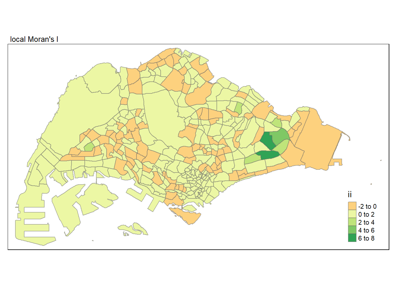
Sign of Local Moran’s I:
Magnitude of Local Moran’s I:
In the code chunk below, tmap functions are used prepare a choropleth map by using value in the p_ii_sim field.
tmap mode set to plotting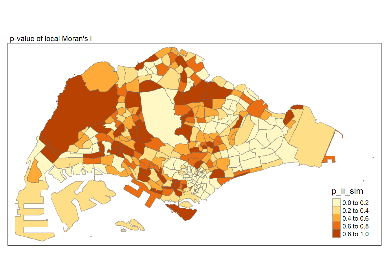
Low P-value (e.g., < 0.05): - Interpretation: A low p-value suggests that the observed spatial pattern is statistically significant. Thus, evidence to reject the null hypothesis that there is no spatial pattern. The observed pattern is likely not due to random chance.
High P-value (e.g., ≥ 0.05): - Interpretation: A high p-value suggests that the observed spatial pattern is not statistically significant. Insufficient evidence to reject the null hypothesis. The observed pattern could be due to random chance.
For effective comparison, it will be better for us to plot both maps next to each other as shown below.
tmap mode set to plottingmap1 <- tm_shape(lisa) +
tm_fill("ii") +
tm_borders(alpha = 0.5) +
tm_view(set.zoom.limits = c(6,8)) +
tm_layout(main.title = "local Moran's I",
main.title.size = 0.8)
map2 <- tm_shape(lisa) +
tm_fill("p_ii",
breaks = c(0, 0.001, 0.01, 0.05, 1),
labels = c("0.001", "0.01", "0.05", "Not sig")) +
tm_borders(alpha = 0.5) +
tm_layout(main.title = "p-value of local Moran's I",
main.title.size = 0.8)
tmap_arrange(map1, map2, ncol = 2)Variable(s) "ii" contains positive and negative values, so midpoint is set to 0. Set midpoint = NA to show the full spectrum of the color palette.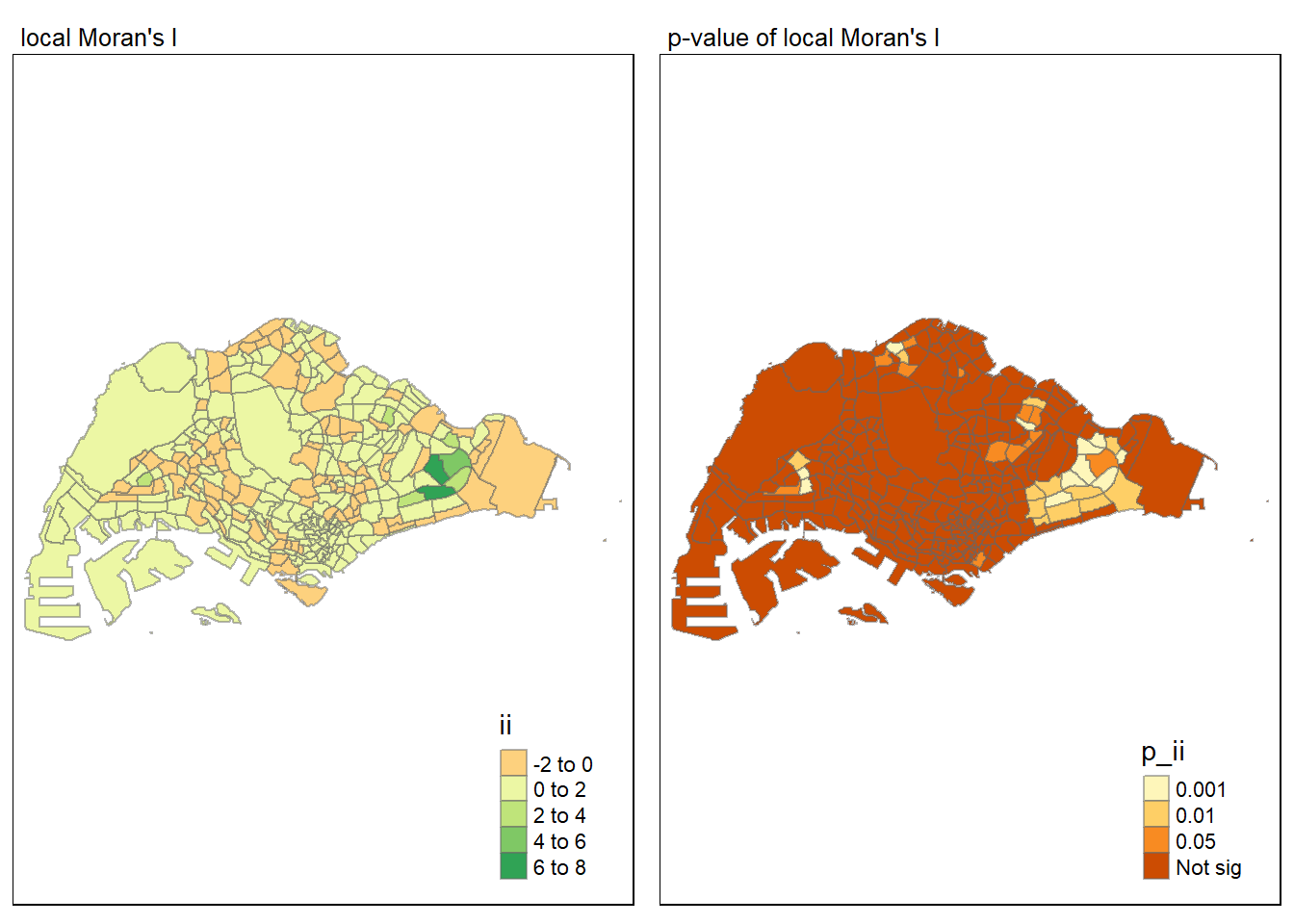
LISA map is a categorical map showing outliers and clusters. There are two types of outliers namely: High-Low and Low-High outliers. Likewise, there are two type of clusters namely: High-High and Low-Low cluaters. In fact, LISA map is an interpreted map by combining local Moran’s I of geographical areas and their respective p-values.
In lisa sf data.frame, we can find three fields contain the LISA categories. They are mean, median and pysal. In general, classification in mean will be used as shown in the code chunk below.
tmap mode set to plottingWarning: One tm layer group has duplicated layer types, which are omitted. To
draw multiple layers of the same type, use multiple layer groups (i.e. specify
tm_shape prior to each of them).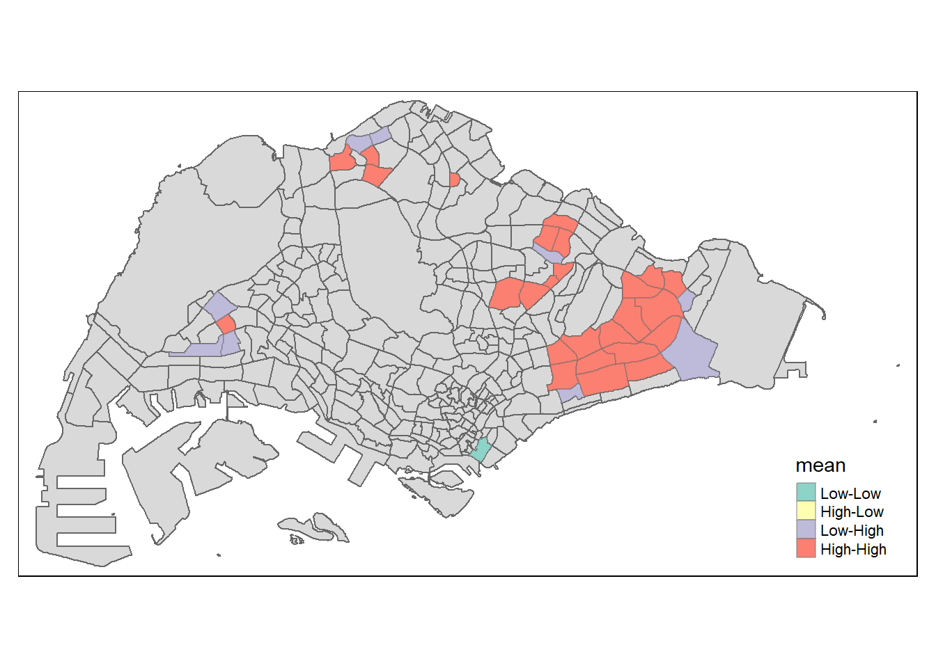
Warning: attribute variables are assumed to be spatially constant throughout
all geometriesvalue_df <- data.frame(
grid_id = intersection_result$grid_id,
TRIPS = intersection_result$TRIPS
)
summarized_values <- aggregate(TRIPS ~ grid_id, value_df, sum)
honeycomb_grid_sf <- merge(honeycomb_grid_sf, summarized_values, by = "grid_id", all.x = TRUE)
honeycomb_grid_sf$n_BS <- ifelse(!is.na(honeycomb_grid_sf$TRIPS), honeycomb_grid_sf$TRIPS, 0)
honeycomb_count <- filter(honeycomb_grid_sf, n_BS > 0)tmap mode set to interactive viewingtm_shape(honeycomb_count) +
tm_fill(
col = "n_BS",
palette = "Reds",
style = "cont",
title = "Distribution of the passenger trips",
id = "grid_id",
showNA = FALSE,
alpha = 0.6,
popup.vars = c(
"Distribution of the passenger trips: " = "n_BS"
),
popup.format = list(
n_BS = list(format = "f", digits = 0)
)
) +
tm_borders(col = "grey40", lwd = 0.7)